Population Genomics Workshop
2019 - NBAF - University of Sheffield
Project maintained by visoca Hosted on GitHub Pages — Theme by mattgraham
Population Genomics Workshop 2019, University of Sheffield
Genetic architecture of traits using multi-locus Genome Wide Association (GWA) mapping with GEMMA
Victor Soria-Carrasco
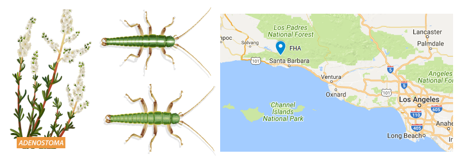
The aim of this practical is use a multi-SNP method to study the genetic architecture of colour pattern phenotype (i.e. white stripe) in Timema cristinae stick insects. In particular, we will use the Bayesian Sparse Linear Mixed Model (BSLMM) model implemented in the program GEMMA, a piece of software that also allow taking into account any potential population structure. This model is a hybrid approach that allows inferring whether the genetic basis of a trait is highly polygenic or rather determined by a few loci (i.e. oligogenic), as well as identifying the loci that show the strongest association with the trait. We will use the dataset of Comeault et al. 2015, which consists of 602 individuals sampled from a phenotypically variable population called FHA. We will infer the proportion of phenotypic variance explained by the genotypes, what fraction of such variance can be explained by a reduced number of major effect loci, and will identify what loci show the most significant association with this trait.
Data and scripts used during this practical will be available in a shared folder in Iceberg, the University of Sheffield HPC cluster, which will allow faster transfers. However, in case attendees would like to use it for practice after the workshop, scripts are also available in this repository and data can be downloaded here (and results here).
Resources
- Zhou et al. 2013 - Paper where the Bayesian Sparse Linear Mixed Model approach implemented in
GEMMAis described. - Zhou Lab website - You can obtain
GEMMAand a few other interesting programs for GWAS here. - GEMMA manual
1. Initial set up
We are going to create a working directory in a dedicated space in the HPC cluster (/data/$USER) and copy the necessary scripts and data files to run this practical.
Connect to Iceberg HPC cluster (change myuser by your username):
ssh myuser@iceberg.sheffield.ac.uk
Request an interactive session:
qrsh
Important note
This tutorial relies on having access to a number of programs. The easiest way is to have your account configured to use the Genomics Software Repository. If that is the case you should see the following message when you get an interactive session with qrsh:
  Your account is set up to use the Genomics Software Repository
     More info: http://soria-carrasco.staff.shef.ac.uk/softrepo
If you don’t get that message, follow the instructions here to set up your account.
In addition, if you want to configure the nano text editor to have syntax highlighting and line numbering, you can configure it this way:
cat /usr/local/extras/Genomics/workshops/February2019/.nanorc >> /home/$USER/.nanorc
Note on transferring output files to your local computer for visualization
You probably will want to transfer files to your own computer for visualization (especially the images). In Linux and Mac, you can do that using rsync on the terminal. For example, to transfer one of the pdf files or all the results that are generated in this practical, the command would be:
# transfer pdf file
rsync myuser@iceberg.sheffield.ac.uk:/data/myuser/gwas_gemma/output/hyperparameters.pdf ./
# transfer all results
rsync -av myuser@iceberg.sheffield.ac.uk:/data/myuser/gwas_gemma/output ./
Another possibility is to email the files, for example:
echo "Text body" | mail -s "Subject: gemma - hyperparameter plot" -a /data/myuser/gwas_gemma/output/hyperparameters.pdf your@email
Graphical alternatives are WinSCP or Cyberduck. You can find more detailed information here.
Change to your data directory:
cd /data/$USER/
Create the working directory for this practical:
mkdir gwas_gemma
Copy scripts:
cp -r /usr/local/extras/Genomics/workshops/February2019/gwas_gemma/scripts ./gwas_gemma
Copy data:
cp -r /usr/local/extras/Genomics/workshops/February2019/gwas_gemma/data ./gwas_gemma/
To check you are getting the expected results, you can also copy a directory containing all the files that should be produced after running this practical:
cp -r /usr/local/extras/Genomics/workshops/February2019/gwas_gemma/results ./gwas_gemma/
Change to the working directory we are going to use for this practical:
cd gwas_gemma
2. Data formatting
Now let’s have a look at the data. You should have the following input files:
ls -lh data
total 1.2G
-rw-r–r– 1 myuser cs 9.9K Jan 28 18:40 fha.pheno
-rw-r–r– 1 myuser cs 1.3K Jan 28 18:40 fha.pheno2
-rw-r–r– 1 myuser cs 876M Jan 28 18:41 fha.vcf.gz
There is a vcf file containing single nucleotide polymorphisms (SNPs) from RAD data of 602 individuals from a single polymorphic population of Timema cristinae (population code FHA). vcf is a very popular format for genetic variants, you can find more info here. You can have a look at the file content with the following commands:
gzip -dc data/fha.vcf.gz | less -S
# or with bcftools
bcftools view data/fha.vcf.gz | less -S
# excluding long header
bcftools view -H data/fha.vcf.gz | less -S
There are two files containing the phenotypes of the same inviduals in the same order than in the vcf file (NA when the phenotype is missing). This phenotypes encode the dorsal white stripe either as a continuous trait (standardised white stripe area; fha.pheno) or as a discerte binary trait (presence/absence of the stripe; fha.pheno2). We will be using the first one for this practical (but it would be a good exercise to repeat analyses using the other one with the probit model using -bslmm 3). You can have a look at the files content:
head data/fha.pheno
0.866078916198945
-1.17516992488642
NA
NA
NA
-3.11627693813939
-0.348977465694598
-0.663007099264362
NA
NA
head data/fha.pheno2
1
1
NA
NA
NA
0
1
1
NA
NA
GEMMA, the program we will be using to carry out multi-variant GWA, needs two input files: one with the genotypes and another one with the phenotypes. Most GWA programs rely on called genotypes, but gemma can work with genotype probabilities, which allows incorporating genotype uncertainty in the analyses. gemma accepts a number of formats for genotypes, we are going to use the mean genotype format (based on the BIMBAM format), where genotypes are encoded as mean genotypes. A mean genotype is a value between 0 and 2 that can be interpreted as the minor allele dosage: 0 is homozygous for the major allele, 1 is a heterozygote, and 2 is a homozygote for the minor allele. Thus, intermediate values reflect the uncertainty in genotypes.
We are going to use the custom Perl script bcf2bbgeno.pl to get such mean genotypes. First, the script removes all the SNPs that have more than two alleles. This is common practice, because most of the models used for inference are based in biallelic variants. Then, the script calculates empirical posterior genotype probabilities from the genotype likelihoods in the vcf file under the assumption that the population is in Hardy-Weinberg equilibrium (HWE). Specifically, the script uses inferred allele frequencies to set HWE priors:
p(AA) = p2; p(aa) = (1-p)2; p(Aa) = 2p(1-p)
being p the allele frequency of major/reference allele A. Genotype likelihoods are multiplied by these priors to obtain genotype posterior probabilities that are then encoded as mean genotypes and saved to a .bbgeno file.
You can get some info about how to run the Perl script:
# show help
scripts/bcf2bbgeno.pl -h
To calculate the genotype posterior probabilites and save them in mean genotype format, we would need to run a command like this one (followed by compression to save some space, given that gemma can handle gzipped files):
scripts/bcf2bbgeno.pl -i data/fha.vcf.gz -o fha.bbgeno -p H-W -s -r
# compress the file to save some space
gzip fha.bbgeno
However, this process may take quite a while (over 1h if the network is slow) and require over the default 2 Gb memory allocated for interactive jobs by default. Therefore it would be better to use submit a batch job to the cluster (see bcf2bbgeno.sh) or, given that it still can take some time, it may be worth to simply skip it altogether and use the .bbgeno.gz and .bbgeno.ids.txt files from the results folder:
cp results/*.bbgeno.* ./
In any case, you should have now two new files: fha.bbgeno.gz, which contains the mean genotypes, and fha.bbgeno.ids.txt, which contains the ids of the samples (i.e. individuals) in the same order as shown in the genotypes file. You can have a look at them:
gzip -dc fha.bbgeno.gz | less -S
lg13_ord45_scaf428-158031 C T 0.01108 0.00279 0.00140 0.00140 0.01108 0.00018 0.01108 0.00555
lg13_ord45_scaf428-48027 T C 0.00299 0.00597 0.00150 0.00019 0.00597 0.00038 0.00009 0.00075
lg13_ord45_scaf428-80879 G A 0.00163 0.00163 0.00325 0.00041 0.00325 0.00041 0.00082 0.00163
lg13_ord45_scaf428-94107 G A 0.00358 0.00358 0.02771 0.01408 0.05530 0.00045 0.01408 0.00358
lg13_ord45_scaf428-158069 T A 0.16220 0.04246 0.02174 0.99552 0.16220 0.00279 0.16220 0.08128
lg13_ord45_scaf428-325672 A T 0.00784 0.00393 0.00197 0.00197 0.00784 0.00099 0.00784 0.00025
The first column is the SNP id, second one is major/reference allele and the third one is the minor/alternate allele. Having major and minor or reference and alternate alleles depends on how you called variants. This does not matter for downstream analyses with gemma, but should be born in mind when interpreting the results. The rest of the columns are the mean genotypes for all the individuals (one for each).
The other file is simply to keep track of the order of the individuals in the genotype file:
less -S fha.bbgeno.ids.txt
2013FHA001
2013FHA002
2013FHA004
2013FHA005
2013FHA006
2013FHA007
3. Running gemma to fit a Bayesian sparse linear mixed model (BSLMM)
gemma, standing for Genome-wide Efficient Mixed Model Association, is a complex piece of software with many options. It is highly recommended that you read carefully the manual. Let’s have a look at the options, with emphasis on the specific ones we will be using.
# general help
gemma -h
# quick guide
gemma -h 1
# input files
gemma -h 2
We will be using the Bayesian sparse linear mixed model (BSLMM):
gemma -h 9
but first we will have to calculate the relatedness matrix to take into account population structure:
gemma -h 8
and it would also be interesting do some filtering such as excluding rare variants, which are difficult to tell apart from sequencing errors:
gemma -h 3
GEMMA uses a relatedness matrix to account for any population structure in the data that may affect results. The easiest way to obtain such matrix is using GEMMA itself. We are going to use the submission script gemma_relmatrix.sh. Let’s have a look with the nano text editor:
nano scripts/gemma_relmatrix.sh
#!/bin/bash
#$ -l h_rt=1:00:00
#$ -j y
#$ -o gemma_relmatrix.log

GEMMA='gemma'
DIR="/data/$USER/gwas_gemma"
GENOTYPES='fha.bbgeno.gz'
PHENOTYPES='data/fha.pheno'
# centered matrix preferred in general, accounts better for population structure
# standardized matrix preferred if SNPs with lower MAF have larger effects
MATRIXTYPE=1 # 1=centered matrix, 2=standardized matrix
OUTBASE='relmatrix'

hostname
uname -a
date
echo "----------------------------------------------------------"
echo
cd $DIR

$GEMMA \
-g $GENOTYPES \
-p $PHENOTYPES \
-gk $MATRIXTYPE \
-o $OUTBASE
echo
echo "----------------------------------------------------------"
date
And then let’s submit the job (it should take just a few minutes):
qsub scripts/gemma_relmatrix.sh
You can check the status of your jobs with Qstat. When finished, it should have two files in the newly created output directory: relmatrix.log.txt, a log file, and relmatrix.cXX.txt, the actual relatedness matrix. If you have a look at them, they should look like these:
cat output/relmatrix.log.txt
##
##GEMMA Version = 0.94
##
##Command Line Input = -g data/fha.bbgeno.gz -p data/fha.pheno -gk 1 -o relmatrix
##
##Summary Statistics:
##number of total individuals = 602
##number of analyzed individuals = 546
##number of covariates = 1
##number of phenotypes = 1
##number of total SNPs = 518232
##number of analyzed SNPs = 346660
##
##Computation Time:
##total computation time = 3.91983 min
##computation time break down:
##time on calculating relatedness matrix = 2.46767 min
##
less -S output/relmatrix.cXX.txt
0.08650617109 0.000333571409 0.001472054408 0.001656484245 0.001901346128 0.001199397691 0.0019
0.000333571409 0.08827073595 0.0008395834056 -0.0008735407094 0.0004308437331 0.004303127573
0.001472054408 0.0008395834056 0.09971276805 0.003820448145 0.001814713502 -0.0001891657497
0.001656484245 -0.0008735407094 0.003820448145 0.10577918 0.002068707695 -7.400802932e-
0.001901346128 0.0004308437331 0.001814713502 0.002068707695 0.05202678922 -8.732093775e-05
0.001199397691 0.004303127573 -0.0001891657497 -7.400802932e-05 -8.732093775e-05
Now we are going to run GEMMA to fit a BSLMM model. Since this will take quite some time (~15 minutes), we are going to submit it as batch job to the cluster queue. We will be using the script gemma_bslmm.sh. We will run GEMMA using the relatedness matrix we estimated before, using the BSLMM model with the continuous phenotypes and excluding variants with a minor allele frequency of lest than 1%. We will run a MCMC chain for 1,000,000 steps, after an initial burn-in of 250,000, saving every 100th step, so that we will end up with 10,000 samples to approximate the posterior distribution of the parameters. Let’s have a look with nano:
nano scripts/gemma_bslmm.sh
#!/bin/bash
#$ -l h_rt=07:00:00
#$ -l rmem=2g
#$ -l mem=4g
#$ -j y
#$ -o gemma_bslmm.log

GEMMA='gemma'

DIR="/data/$USER/gwas_gemma"
GENOTYPES='fha.bbgeno.gz'
PHENOTYPES='data/fha.pheno'
RELMATRIX='output/relmatrix.cXX.txt'
BSLMM=1 # 1=BSLMM, 2=standard ridge regression/GBLUP (no mcmc), 3=probit BSLMM (requires 0/1 phenotypes)
OUTBASE='bslmm'

# Number of variants that will be used (required for setting some priors and proposals below)
NVARS=$(grep "number of analyzed SNPs" $DIR/output/relmatrix.log.txt | perl -pe 's/.*\= //g')

# priors
# ----------------
# h -> approximation to PVE: proportion of phenotypic variance explained by loci
HMIN=0
HMAX=1

# rho -> approximation to PGE: proportion of genetic variance explained by sparse effect terms (~major effect loci)
# rho=0 -> pure LMM, highly polygenic; rho=1 => pure BVSR, few loci
RHOMIN=0
RHOMAX=1

# pi -> proportion of variants with non-zero effects (random + sparse effects)
PIMIN=$(Rscript -e 'cat(log10(1/'$NVARS'))') # log10(1/no_variants)
PIMAX=0 # log10(1)

# gamma -> Number of variants with sparse effects (~ number of major effect loci)
GAMMAMIN=0
GAMMAMAX=300
# ----------------

# proposals
# ----------------
# don't need to tweak them unless you have convergence problems
GEOMMEAN=2000
HSTEP=$(Rscript -e 'cat(min(c(10/sqrt('$NVARS'),1)))') # 0-1, default: min(10/sqrt(no_variants),1)
RHOSTEP=$(Rscript -e 'cat(min(c(10/sqrt('$NVARS'),1)))') # 0-1, default: min(10/sqrt(no_variants),1)
PISTEP=$(Rscript -e 'cat(min(c(5/sqrt('$NVARS'),1)))') # 0-1, default: min(5/sqrt(n),1)
# ----------------

# chain parameters
# ----------------
BURNIN=250000 # No MCMC initial steps to be discarded (suggested: 10-25% MCCMC length)
MCMCLEN=1000000 # No MCMC steps after burnin
RECORDPACE=100 # Record states every X steps
WRITEPACE=1000 # Write to file every X steps (suggested: >=MCMCLEN/1000)
# ----------------

# QC filters
# ----------------
MAF='0.01' # exclude very rare variants
# ----------------

hostname
uname -a
date
echo "----------------------------------------------------------"
echo
cd $DIR

$GEMMA \
-g $GENOTYPES \
-p $PHENOTYPES \
-k $RELMATRIX \
-bslmm $BSLMM \
-w $BURNIN \
-s $MCMCLEN \
-rpace $RECORDPACE \
-wpace $WRITEPACE \
-maf $MAF \
-o $OUTBASE

# This is a commented example in case you would like
# to specify specify priors and proposals
# $GEMMA \
# -g $GENOTYPES \
# -p $PHENOTYPES \
# -k $RELMATRIX \
# -bslmm $BSLMM \
# -hmin $HMIN \
# -hmax $HMAX \
# -rmin $RHOMIN \
# -rmax $RHOMAX \
# -pmin $PIMIN \
# -pmax $PIMAX \
# -gmean $GEOMMEAN \
# -hscale $HSTEP \
# -rscale $RHOSTEP \
# -pscale $PISTEP \
# -w $BURNIN \
# -s $MCMCLEN \
# -rpace $RECORDPACE \
# -wpace $WRITEPACE \
# -maf $MAF \
# -o $OUTBASE

echo
echo "----------------------------------------------------------"
date
Let’s submit the job to the queue:
qsub scripts/gemma_bslmm.sh
Run time should be around 15 minutes. You can check if the job has finished with Qstat. When finished, we should have the following files in the output folder:
ls -lh output
-rw-r–r– 1 myuser cs 7.4K Jan 29 13:17 bslmm.bv.txt
-rw-r–r– 1 myuser cs 6.0M Jan 29 13:17 bslmm.gamma.txt
-rw-r–r– 1 m 29 13:17 bslmm.hyp.txt
-rw-r–r– 1 myuser cs 1.3K Jan 29 13:17 bslmm.log.txt
-rw-r–r– 1 myuser cs 25M Jan 29 13:17 bslmm.param.txt
-rw-r–r– 1 myuser cs 5.7M Jan 29 12:55 relmatrix.cXX.txt
-rw-r–r– 1 myuser cs 505 Jan 29 12:55 relmatrix.log.txt
The new files generated are:
- bslmm.bv.txt -> posterior samples of breeding values (~estimated random effects)
- bslmm.gamma.txt -> posterior samples of gamma (i.e. sparse effects) listing the SNPs included in the model in each iteration, that is the loci with detectable (large) effects
- bslmm.hyp.txt -> posterior samples of hyperparameters, including the proportion of the variance explained (pve), the proportion of the genetic variance (i.e. pve) explained by the sparse effect loci (pge), the proportion of SNPs with non-zero effects (pi) and the estimated number of loci with large effects (n_gamma)
- bslmm.log.txt -> log file
- bslmm.param.txt -> posterior samples of parameters: random effects (alpha), fixed effects (beta), and sparse effects (gamma)
Let’s have a look at the log. Notice the number of individuals with both genotypic and phenotypic data is 546 out of 602 and the number of SNPs was reduced from 518,232 to 346,660 after excluding SNPs missing genotypes for over 5% individuals default threshold) and rare variants (minor allele frequency of less than 1%):
less -S output/bslmm.log.txt
##
##GEMMA Version = 0.94
##
##Command Line Input = -g data/fha.bbgeno.gz -p data/fha.pheno -k output/relmatrix.cXX.txt -bslmm 1 -w 250000 -s 1000000 -rpace 100 -wpace 1000 -maf 0.01 -o bslmm
##
##Summary Statistics:
##number of total individuals = 602
##number of analyzed individuals = 546
##number of covariates = 1
##number of phenotypes = 1
##number of total SNPs = 518232
##number of analyzed SNPs = 346660
##REMLE log-likelihood in the null model = -737.564
##MLE log-likelihood in the null model = -737.31
##pve estimate in the null model = 0.889028
##se(pve) in the null model = 0.0499207
##vg estimate in the null model = 0
##ve estimate in the null model = 0
##beta estimate in the null model =
##se(beta) =
##estimated mean = 1.17936e-16
##
##MCMC related:
##initial value of h = 0.889028
##initial value of rho = 0.626463
##initial value of pi = 0.000865401
##initial value of |gamma| = 300
##random seed = 47472
##acceptance ratio = 0.122066
##
##Computation Time:
##total computation time = 14.2177 min
##computation time break down:
##time on calculating relatedness matrix = 0 min
##time on eigen-decomposition = 0.00716667 min
##time on calculating UtX = 2.52367 min
##time on mcmc = 9.01583 min
##time on Omega = 2.15233 min
##
the hyperparameters:
less -S output/bslmm.hyp.txt
h pve rho pge pi n_gamma
5.679255e-01 5.827644e-01 4.814629e-01 5.298608e-01 1.708291e-05 3
4.568325e-01 5.845055e-01 3.623301e-01 6.121603e-01 1.639111e-05 5
5.652819e-01 6.551080e-01 4.100889e-01 5.755021e-01 1.543192e-05 6
6.076860e-01 5.368049e-01 6.785772e-01 5.821440e-01 1.722759e-05 3
5.805904e-01 4.711531e-01 8.102496e-01 6.904983e-01 1.388330e-05 3
and the parameters (notice we didn’t specify chromosome nor positions and therefore there are only SNP ids, i.e. rs):
less -S output/bslmm.param.txt
chr rs ps n_miss alpha beta gamma
-9 lg13_ord45_scaf428-94107 -9 0 2.887084e-05 0.000000e+00 0.000000e+00
-9 lg13_ord45_scaf428-158069 -9 0 -1.256153e-05 0.000000e+00 0.000000e+00
-9 lg13_ord45_scaf428-466300 -9 0 1.338440e-05 0.000000e+00 0.000000e+00
-9 lg13_ord45_scaf428-337230 -9 0 1.912454e-05 0.000000e+00 0.000000e+00
-9 lg13_ord45_scaf428-351513 -9 0 -5.619149e-05 0.000000e+00 0.000000e+00
4. Analysing gemma BSLMM output
We will use two R scripts to analyse GEMMA output and produce some plots. These scripts can be run in batch mode like executing: Rscript gemma_hyperparam.R, but you are likely to learn much more if you follow the steps below to run them step by step. Bear in mind the rest of the practical is only R code and will have to run within an R session. Open an R session simply typing the command R.
First, we are going to play with the hyperparameter estimates, which will inform us of the genetic architecture of the trait. This is the script gemma_hyperparam.R.
First we change the working directory:
user<-Sys.getenv("USER")
wkpath<-paste("/data/",user, "/gwas_gemma/output",sep="")
setwd(wkpath)
And then load the hyperparameter file:
# Load hyperparameter file
# ==============================================================================
hyp.params<-read.table("bslmm.hyp.txt",header=T)
# ==============================================================================
Let’s get some statistics (mean, median, and 95% ETPI):
# Get mean, median, and 95% ETPI of hyperparameters
# ==============================================================================
# pve -> proportion of phenotypic variance explained by the genotypes
pve<-c("PVE", mean(hyp.params$pve),quantile(hyp.params$pve, probs=c(0.5,0.025,0.975)))

# pge -> proportion of genetic variance explained by major effect loci
pge<-c("PGE",mean(hyp.params$pge),quantile(hyp.params$pge, probs=c(0.5,0.025,0.975)))

# pi -> proportion of variants with non-zero effects
pi<-c("pi",mean(hyp.params$pi),quantile(hyp.params$pi, probs=c(0.5,0.025,0.975)))

# n.gamma -> number of variants with major effect
n.gamma<-c("n.gamma",mean(hyp.params$n_gamma),quantile(hyp.params$n_gamma, probs=c(0.5,0.025,0.975)))
# ==============================================================================

# get table of hyperparameters
# ==============================================================================
hyp.params.table<-as.data.frame(rbind(pve,pge,pi,n.gamma),row.names=F)
colnames(hyp.params.table)<-c("hyperparam", "mean","median","2.5%", "97.5%")
# show table
hyp.params.table
# write table to file
write.table(hyp.params.table, file="hyperparameters.dsv", sep="\t", quote=F)
# ==============================================================================
Values should be similar to this:
| hyperparam | mean | median | 2.5% | 97.5% |
|---|---|---|---|---|
| PVE | 0.50758534164 | 0.49616535 | 0.3290844075 | 0.753359795 |
| PGE | 0.70427977221 | 0.70412075 | 0.4118065175 | 0.9789640325 |
| pi | 1.29564889986e-05 | 9.376132e-06 | 3.25441665e-06 | 4.3316011e-05 |
| n.gamma | 4.574 | 4 | 1 | 14 |
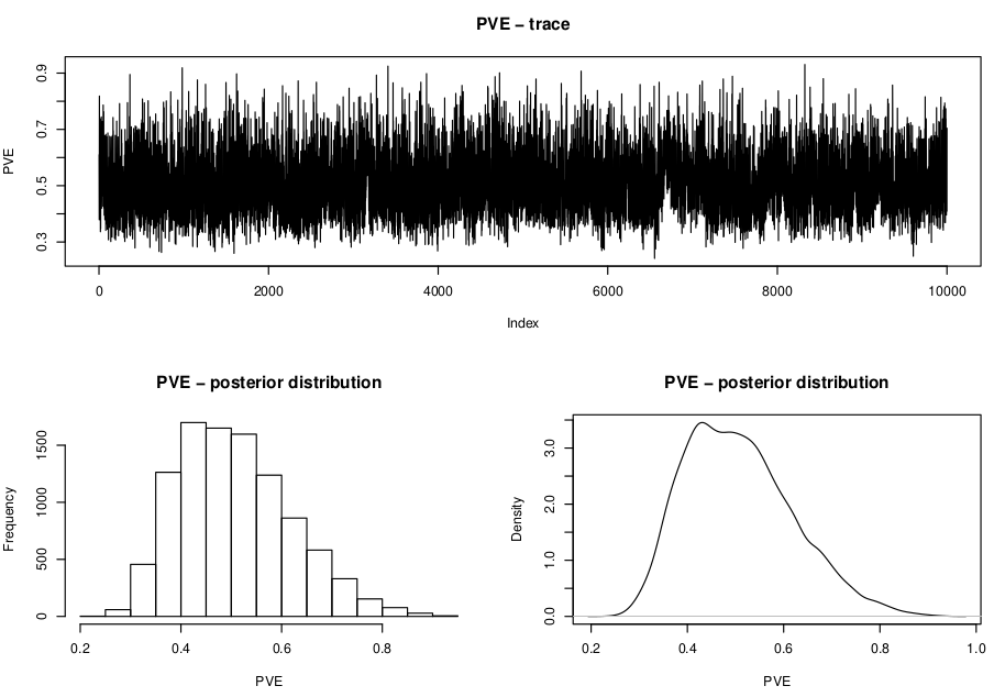
Now let’s plot the MCMC traces and the posterior distributions of the hyperparameters and save them into a pdf file.
# plot traces and distributions of hyperparameters
# ==============================================================================
pdf(file="hyperparameters.pdf", width=8.3,height=11.7)
layout(matrix(c(1,1,2,3,4,4,5,6), 4, 2, byrow = TRUE))

# PVE
# ------------------------------------------------------------------------------
plot(hyp.params$pve, type="l", ylab="PVE", main="PVE - trace")
hist(hyp.params$pve, main="PVE - posterior distribution", xlab="PVE")
plot(density(hyp.params$pve), main="PVE - posterior distribution", xlab="PVE")
# ------------------------------------------------------------------------------

# PGE
# ------------------------------------------------------------------------------
plot(hyp.params$pge, type="l", ylab="PGE", main="PGE - trace")
hist(hyp.params$pge, main="PGE - posterior distribution", xlab="PGE")
plot(density(hyp.params$pge), main="PGE - posterior distribution", xlab="PGE")
# ------------------------------------------------------------------------------

# pi
# ------------------------------------------------------------------------------
plot(hyp.params$pi, type="l", ylab="pi", main="pi")
hist(hyp.params$pi, main="pi", xlab="pi")
plot(density(hyp.params$pi), main="pi", xlab="pi")
# ------------------------------------------------------------------------------

# No gamma
# ------------------------------------------------------------------------------
plot(hyp.params$n_gamma, type="l", ylab="n_gamma", main="n_gamma - trace")
hist(hyp.params$n_gamma, main="n_gamma - posterior distribution", xlab="n_gamma")
plot(density(hyp.params$pi), main="n_gamma - posterior distribution", xlab="n_gamma")
# ------------------------------------------------------------------------------
dev.off()
# ==============================================================================
Ideally, the MCMC traces should look like a caterpillar and distributions should be generally unimodal, indicating that mixing was good. Also it is highly recommended to run GEMMA multiple times (at least 3) and compare both the traces and the posterior distributions of the hyperparameters obtained from different runs and check that all are converging into the same values. However, we will not do this in this practical for time reasons. For instance, PVE should look like this:
We are going to study now the parameter estimates to see if there are SNPs strongly and consistenly associated with the trait. We are going to use the script gemma_param.R. As before, we are going to use an R interactive session to go through it step by step.
Let’s change to the working directory (this might not be necessary if you are using the same R session than before):
# change to the working directory
user<-Sys.getenv("USER")
wkpath<-paste("/data/",user, "/gwas_gemma/output",sep="")
setwd(wkpath)
We will load a library to speed the loading of large tables to memory and will load the parameter estimates:
# library to speed up loading of big tables
library(data.table)

# Load parameters output
# ==============================================================================
params<-fread("bslmm.param.txt",header=T,sep="\t", data.table=F)
# ==============================================================================
Now we will get the SNPs that have a sparse effect (i.e. detectable large effect) on the phenotype. In the table, beta is actually β|γ == 1 for given SNP, being β the small effect all variants have and γ the additional large effect only some variants have. Thus, the sparse effect size for each SNP is calculated multiplying β by γ.
# Get variants with sparse effect size on phenotypes
# ==============================================================================
# add sparse effect size (= beta * gamma) to data frame
params["eff"]<-abs(params$beta*params$gamma)
Then we get the SNPs that have a detectable large effect size, sort them by effect size, and save the top SNPs using several thresholds (1%, 0.1%, 0.01%):
# get variants with effect size > 0
params.effects<-params[params$eff>0,]

# show number of variants with measurable effect
nrow(params.effects)

# sort by descending effect size
params.effects.sort<-params.effects[order(-params.effects$eff),]

# show top 10 variants with highest effect
head(params.effects.sort, 10)

# variants with the highest sparse effects
# ------------------------------------------------------------------------------
# top 1% variants (above 99% quantile)
top1<-params.effects.sort[params.effects.sort$eff>quantile(params.effects.sort$eff,0.99),]
# top 0.1% variants (above 99.9% quantile)
top01<-params.effects.sort[params.effects.sort$eff>quantile(params.effects.sort$eff,0.999),]
# top 0.01% variants (above 99.99% quantile)
top001<-params.effects.sort[params.effects.sort$eff>quantile(params.effects.sort$eff,0.9999),]
# ------------------------------------------------------------------------------

# write tables
write.table(top1, file="top1eff.dsv", quote=F, row.names=F, sep="\t")
write.table(top01, file="top0.1eff.dsv", quote=F, row.names=F, sep="\t")
write.table(top001, file="top0.01eff.dsv", quote=F, row.names=F, sep="\t")
There should be around 15595 SNPs with detectable sparse effects and the top SNPs should look like this (notice we didn’t specify chromosome nor positions and therefore there are only SNP ids, i.e. rs):
| chr | rs | ps | n_miss | alpha | beta | gamma | |||
|---|---|---|---|---|---|---|---|---|---|
| -9 | lg8_ord45_scaf1036-131573 | -9 | 0 | -1.229901e-05 | -1.2065980 | 0.5364 | 4929 | 0.64721917 | |
| -9 | lg8_ord55_scaf1512-149001 | -9 | 0 | -6.640361e-05 | -0.7905428 | 0.5635 | 4943 | 0.48103043 | |
| -9 | lg8_ord66_scaf318-448145 | -9 | 0 | -1.133074e-04 | -0.6136137 | 0.0566 | 341474 | 0.44547087 | |
| -9 | lgNA_ordNA_scaf784-237602 | -9 | 0 | 1.004314e-04 | 0.7119540 | 0.0378 | 330495 | 0.03473054 | |
| -9 | lg3_ord81_scaf488-29866 | -9 | 0 | 7.241678e-05 | 0.9273204 | 0.0232 | 315197 | 0.02691186 | |
| -9 | lgNA_ordNA_scaf154-274617 | -9 | 0 | 5.164412e-05 | 1.1116970 | 0.0157 | 5105 | 0.02151383 | |
| -9 | lg6_ord32_scaf531-110990 | -9 | 0 | 6.656697e-05 | 0.9619961 | 0.0169 | 183101 | 0.01745364 | |
| -9 | lg6_ord32_scaf531-110990 | -9 | 0 | 6.656697e-05 | 0.9619961 | 0.0169 | 138641 | 0.01625773 | |
| -9 | lg6_ord32_scaf531-110989 | -9 | 0 | 6.606357e-05 | 0.9763403 | 0.0144 | 138636 | 0.01405930 | |
| -9 | lg3_ord28_scaf970-18573 | -9 | 0 | 5.868428e-05 | 1.1262150 | 0.0109 | 138636 | 0.01405930 | 0.01227574 |
We are going to estimate the Posterior Inclusion Probability (PIP), that is the frequency a SNP is estimated to have a detectable large effect in the MCMC (i.e. γ). This can be used as a measure of the strength of association of a SNP with a phenotype. As with the effect sizes we will sort them by PIP, and save the top SNPs using several thresholds (0.01, 0.1, 0.25, 0.5):
# ==============================================================================
# Get variants with high Posterior Inclusion Probability (PIP) == gamma
# ==============================================================================
# PIP is the frequency a variant is estimated to have a sparse effect in the MCMC

# sort variants by descending PIP
params.pipsort<-params[order(-params$gamma),]

# Show top 10 variants with highest PIP
head(params.pipsort,10)

# sets of variants above a certain threshold
# variants with effect in 1% MCMC samples or more
pip01<-params.pipsort[params.pipsort$gamma>=0.01,]
# variants with effect in 10% MCMC samples or more
pip10<-params.pipsort[params.pipsort$gamma>=0.10,]
# variants with effect in 25% MCMC samples or more
pip25<-params.pipsort[params.pipsort$gamma>=0.25,]
# variants with effect in 50% MCMC samples or more
pip50<-params.pipsort[params.pipsort$gamma>=0.50,]

# write tables
write.table(pip01, file="pip01.dsv", quote=F, row.names=F, sep="\t")
write.table(pip10, file="pip10.dsv", quote=F, row.names=F, sep="\t")
write.table(pip25, file="pip25.dsv", quote=F, row.names=F, sep="\t")
write.table(pip50, file="pip50.dsv", quote=F, row.names=F, sep="\t")
# ------------------------------------------------------------------------------
You can see the SNPs are very similar but not exactly the same ones than when sorted by effect size:
| chr | rs | ps | n_miss | alpha | beta | gamma | |
|---|---|---|---|---|---|---|---|
| -9 | lg8_ord55_scaf1512-149001 | -9 | 0 | -6.640361e-05 | -0.7905428 | 0.5635 | 0.445470868 |
| -9 | lg8_ord45_scaf1036-131573 | -9 | 0 | -1.229901e-05 | -1.2065980 | 0.5364 | 0.647219167 |
| -9 | lg8_ord45_scaf1036-131605 | -9 | 0 | -1.096165e-05 | -1.0375980 | 0.4636 | 0.481030433 |
| -9 | lg8_ord66_scaf318-448145 | -9 | 0 | -1.133074e-04 | -0.6136137 | 0.0566 | 0.034730535 |
| -9 | lgNA_ordNA_scaf784-237602 | -9 | 0 | 1.004314e-04 | 0.7119540 | 0.0378 | 0.026911861 |
| -9 | lg1_ord96_scaf190-725578 | -9 | 0 | -2.183769e-04 | -0.3418733 | 0.0326 | 0.011145070 |
| -9 | lg3_ord81_scaf488-29866 | -9 | 0 | 7.241678e-05 | 0.9273204 | 0.0232 | 0.021513833 |
| -9 | lg10_ord64_scaf380-30883 | -9 | 0 | -2.363161e-04 | -0.3245005 | 0.0180 | 0.005841009 |
| -9 | lg8_ord60_scaf2482-78371 | -9 | 0 | 1.514078e-04 | 0.4569336 | 0.0174 | 0.007950645 |
| -9 | lg6_ord32_scaf531-110990 | -9 | 0 | 6.656697e-05 | 0.9619961 | 0.0169 | 0.016257734 |
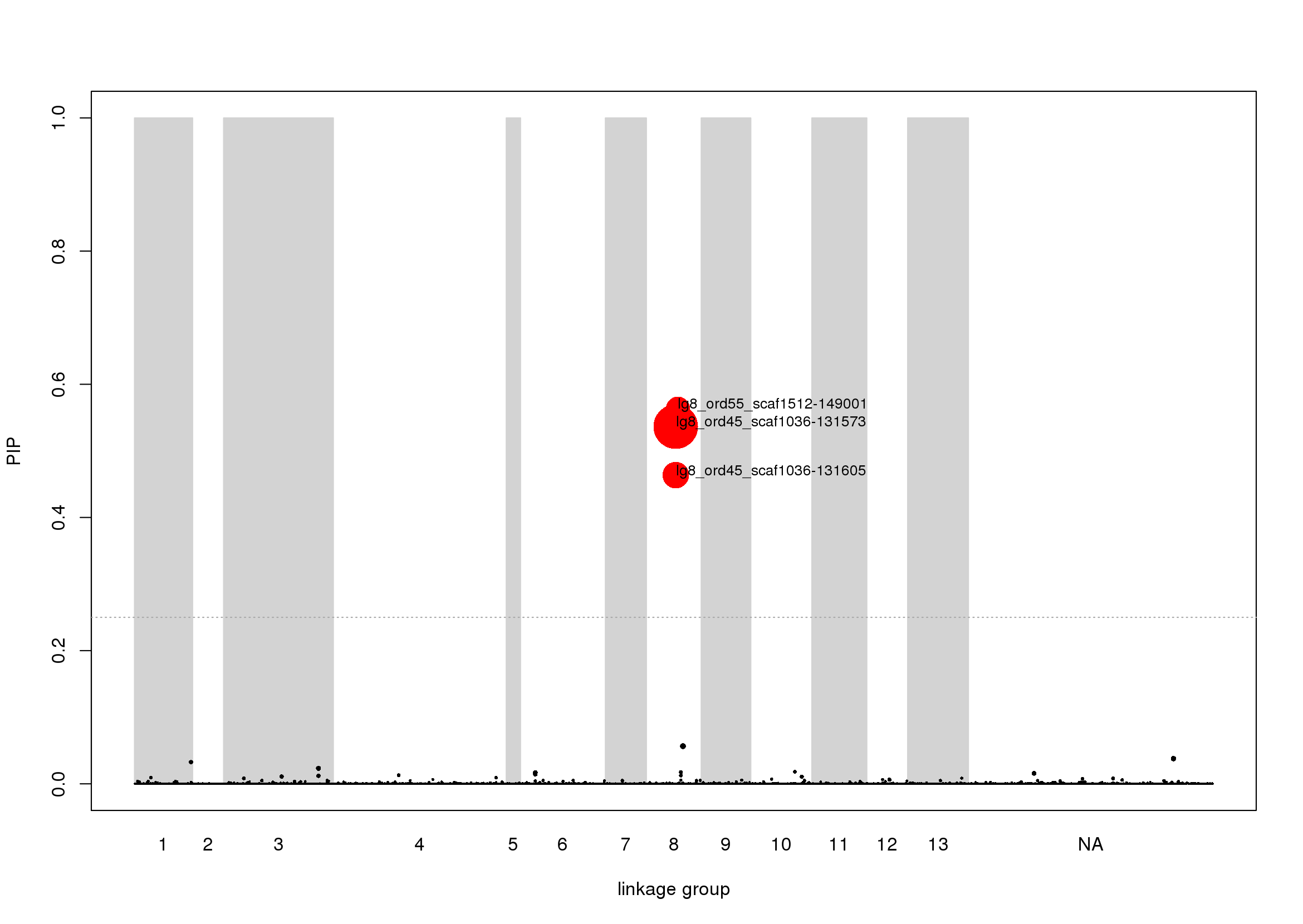
Lastly we can generate a Manhattan plot of the PIPs to visualize the distribution of associated SNPs across the genome and save it as a png file. We will highlight the top candidates in the genome and make the size of the dots reflect the effect size.
# ==============================================================================
# plot variants PIPs across linkage groups/chromosomes
# ==============================================================================
# Prepare data
# ------------------------------------------------------------------------------
# add linkage group column (chr)
chr<-gsub("lg|_.+","",params$rs)
params["chr"]<-chr

# sort by linkage group and position
params.sort<-params[order(as.numeric(params$chr), params$rs),]

# get list of linkage groups/chromosomes
chrs<-sort(as.numeric(unique(chr)))
# ------------------------------------------------------------------------------

# Plot to a png file because the number of dots is very high
# drawing this kind of plot over the network is very slow
# also opening vectorial files with many objects is slow
# ------------------------------------------------------------------------------
# ------------------------------------------------------------------------------
png(file="pip_plot.png", width=11.7,height=8.3,units="in",res=200)

# set up empty plot
plot(-1,-1,xlim=c(0,nrow(params.sort)),ylim=c(0,1),ylab="PIP",xlab="linkage group", xaxt="n")


# plot grey bands for chromosome/linkage groups
# ------------------------------------------------------------------------------
start<-1
lab.pos<-vector()
for (ch in chrs){
  size<-nrow(params.sort[params.sort$chr==ch,])
  cat ("CH: ", ch, "\n")
  colour<-"light grey"
  if (ch%%2 > 0){
    polygon(c(start,start,start+size,start+size,start), c(0,1,1,0,0), col=colour, border=colour)
  }
  cat("CHR: ", ch, " variants: ", size, "(total: ", (start+size), ")\n")
  txtpos<-start+size/2
  lab.pos<-c(lab.pos, txtpos)

  start<-start+size
}
# Add variants outside linkage groups
chrs<-c(chrs,"NA")
size<-nrow(params.sort[params.sort$chr=="NA",])
lab.pos<-c(lab.pos, start+size/2)
# ------------------------------------------------------------------------------

# Add x axis labels
axis(side=1,at=lab.pos,labels=chrs,tick=F)

# plot PIP for all variants
# ------------------------------------------------------------------------------
# rank of variants across linkage groups
x<-seq(1,length(params.sort$gamma),1)
# PIP
y<-params.sort$gamma
# sparse effect size, used for dot size
z<-params.sort$eff
# log-transform to enhance visibility
z[z==0]<-0.00000000001
z<-1/abs(log(z))
# plot
symbols(x,y,circles=z, bg="black",inches=1/5, fg=NULL,add=T)
# ------------------------------------------------------------------------------

# highligh high PIP variants (PIP>=0.25)
# ------------------------------------------------------------------------------
# plot threshold line
abline(h=0.25,lty=3,col="dark grey")
# rank of high PIP variants across linkage groups
x<-match(params.sort$gamma[params.sort$gamma>=0.25],params.sort$gamma)
# PIP
y<-params.sort$gamma[params.sort$gamma>=0.25]
# sparse effect size, used for dot size
z<-params.sort$eff[params.sort$gamma>=0.25]
z<-1/abs(log(z))

symbols(x,y,circles=z, bg="red",inches=1/5,fg=NULL,add=T)
# ------------------------------------------------------------------------------

# add label high PIP variants
text(x,y,labels=params.sort$rs[params.sort$gamma>=0.25], adj=c(0,0), cex=0.8)
# ------------------------------------------------------------------------------
# ------------------------------------------------------------------------------

# close device
dev.off()
# ==============================================================================
The PIP plot shows there are three large effect size SNPs strongly associated with colour pattern in two non-contiguous scaffolds that belong to linkage group 8:
Remember to quit the R session when finished:
quit()