SNP and genotype calling

Population structure with NGSadmix

NGSadmix is a programme (part of the package ANGSD) for inferring admixture from genotype likelihoods, thus taking into account the uncertainty inherent to NGS data. It is similar to the famous programme STRUCTURE, but better suited for low-coverage NGS data. For those not familiar with this kind of approaches, these programmes allow investigating population structure by inferring individual admixture proportions given a number of populations. This allows also assigning individuals to populations and identifying migrants or admixed individuals.

We first need to conver the bcf file to beagle format with angsd:

mkdir ngsadmix
angsd -vcf-gl <(bcftools view -O v filtering/snps.bcf) -fai genome/Hmel2.fa.fai -doMaf 3 -nInd 32 -domajorminor 1 -doglf 2 -out ngsadmix/snps

Now prepare the script to run NGSadmix for K=2 to K=4 in parallel, using 2 cores for each task:

#!/bin/bash
#$ -l h_rt=1:00:00
#$ -l mem=2G
#$ -t 1-4
#$ -pe smp 2
#$ -m bea
#$ -M myemail@mail.com
#$ -j y
#$ -o ngsadmix.log
#$ -N ngsadmix

# internal SGE task index
K=$(($SGE_TASK_ID+1))

# log file
LOG=ngsadmix/snps_K$K.sclog

# Redirect all the following screen outputs to log file
exec > $LOG 2>&1

hostname
date
echo "=============================================================================="

# Load genomics software repository
# (safer to load it here in case the worker nodes don't inherit the environment)
source /usr/local/extras/Genomics/.bashrc 

NGSadmix \
-P 2 \
-likes ngsadmix/snps.beagle.gz \
-K $K \
-o ngsadmix/snps_K$K 

echo "=============================================================================="
date

When you have finished editing the bash script, save it as ngsadmix.sh, make it executable with chmod and submit it to the job queue with qsub:

chmod +x ngsadmix.sh
qsub ngsadmix.sh

After running, you should have the following files:

ls -lh ngsadmix

total 136K
-rw-r--r-- 1 bo1vsx bo 7.0K Feb 18 04:29 snps.arg
-rw-r--r-- 1 bo1vsx bo 16K Feb 18 04:29 snps.beagle.gz
-rw-r--r-- 1 bo1vsx bo 0 Feb 18 04:29 snps_K2.filter
-rw-r--r-- 1 bo1vsx bo 7.1K Feb 18 04:29 snps_K2.fopt.gz
-rw-r--r-- 1 bo1vsx bo 491 Feb 18 04:29 snps_K2.log
-rw-r--r-- 1 bo1vsx bo 1.5K Feb 18 04:29 snps_K2.qopt
-rw-r--r-- 1 bo1vsx bo 1.3K Feb 18 04:29 snps_K2.sclog
-rw-r--r-- 1 bo1vsx bo 0 Feb 18 04:29 snps_K3.filter
-rw-r--r-- 1 bo1vsx bo 9.6K Feb 18 04:29 snps_K3.fopt.gz
-rw-r--r-- 1 bo1vsx bo 491 Feb 18 04:29 snps_K3.log
-rw-r--r-- 1 bo1vsx bo 2.2K Feb 18 04:29 snps_K3.qopt
-rw-r--r-- 1 bo1vsx bo 1.2K Feb 18 04:29 snps_K3.sclog
-rw-r--r-- 1 bo1vsx bo 0 Feb 18 04:29 snps_K4.filter
-rw-r--r-- 1 bo1vsx bo 14K Feb 18 04:29 snps_K4.fopt.gz
-rw-r--r-- 1 bo1vsx bo 491 Feb 18 04:29 snps_K4.log
-rw-r--r-- 1 bo1vsx bo 3.0K Feb 18 04:29 snps_K4.qopt
-rw-r--r-- 1 bo1vsx bo 1.3K Feb 18 04:29 snps_K4.sclog
-rw-r--r-- 1 bo1vsx bo 0 Feb 18 04:29 snps_K5.filter
-rw-r--r-- 1 bo1vsx bo 17K Feb 18 04:29 snps_K5.fopt.gz
-rw-r--r-- 1 bo1vsx bo 491 Feb 18 04:29 snps_K5.log
-rw-r--r-- 1 bo1vsx bo 3.7K Feb 18 04:29 snps_K5.qopt
-rw-r--r-- 1 bo1vsx bo 1.3K Feb 18 04:29 snps_K5.sclog
-rw-r--r-- 1 bo1vsx bo 5.1K Feb 18 04:29 snps.mafs.gz

The ones we are interested on here are the .qopt files that contain the admixture proportions:

head ngsadmix/snps_K2.qopt

should show something like:

0.99999999900000002828 0.00000000100000000000
0.91360213481999608121 0.08639786518000389104
0.99999999900000002828 0.00000000100000000000
0.99999999900000002828 0.00000000100000000000
0.50578260909553407476 0.49421739090446586973
0.51391688264848356393 0.48608311735151649158
0.00000000100000000000 0.99999999900000002828
0.00000000100000000000 0.99999999900000002828
0.99999999900000002828 0.00000000100000000000
0.99999999900000002828 0.00000000100000000000

Now we are going to visualize the admixture estimates using ´R´. We will need some more information about the samples to produce meaningful plots. A file with information about the race and the sex of each sample can be copied from a shared directory on ShARC:

cp /usr/local/extras/Genomics/workshops/NGS_AdvSta_2019/SNPgenocall/sample_race_sex.tsv ngsadmix/ 
head ngsadmix/sample_race_sex.tsv

Now, let’s launch an interactive session of R and generate some plots for the admixture inferences when K=2. When you launch R:

you should see something like this:

R version 3.4.3 (2017-11-30) -- "Kite-Eating Tree"
Copyright (C) 2017 The R Foundation for Statistical Computing
Platform: x86_64-pc-linux-gnu (64-bit)

R is free software and comes with ABSOLUTELY NO WARRANTY.
You are welcome to redistribute it under certain conditions.
Type 'license()' or 'licence()' for distribution details.

Natural language support but running in an English locale

R is a collaborative project with many contributors.
Type 'contributors()' for more information and
'citation()' on how to cite R or R packages in publications.

Type 'demo()' for some demos, 'help()' for on-line help, or
'help.start()' for an HTML browser interface to help.
Type 'q()' to quit R.

>

Now let’s load the admixture proportions, the information about the individuals, and let’s do some plotting:

# Load admixture proportions
admix<-t(as.matrix(read.table("ngsadmix/snps_K2.qopt")))

# Load info about samples
id.info<-read.table("ngsadmix/sample_race_sex.tsv", sep="\t", header=T)

# Add category combining race and sex
id.info['race.sex']<-paste(id.info$race,id.info$sex,sep="-")

# Palette for plotting
mypal<-c("#E41A1C","#377EB8","#4DAF4A","#984EA3")

# sort by race and plot
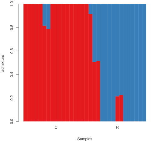
admix<-admix[,order(id.info$race)]
id.info<-id.info[order(id.info$race),]

pdf(file="ngsadmix/snps_K2_byrace.pdf")
h<-barplot(admix,col=mypal,space=0,border=NA,xlab="Samples",ylab="admixture")
text(tapply(1:nrow(id.info),id.info$race,mean),-0.05,unique(id.info$race),xpd=T)
dev.off()

# sort by sex
admix<-admix[,order(id.info$sex)]
id.info<-id.info[order(id.info$sex),]

pdf(file="ngsadmix/snps_K2_bysex.pdf")
h<-barplot(admix,col=mypal,space=0,border=NA,xlab="Samples",ylab="admixture")
text(tapply(1:nrow(id.info),id.info$sex,mean),-0.05,unique(id.info$sex),xpd=T)
dev.off()

# sort by race and sex
admix<-admix[,order(id.info$race.sex)]
id.info<-id.info[order(id.info$race.sex),]

pdf(file="ngsadmix/snps_K2_byracebysex.pdf")
h<-barplot(admix,col=mypal,space=0,border=NA,xlab="Samples",ylab="admixture")
text(tapply(1:nrow(id.info),id.info$race.sex,mean),-0.05,unique(id.info$race.sex),xpd=T)
dev.off()

This generates 3 pdf files that can be downloaded for visualization. For example, for race, it should look like this:

snps_K2_byrace

Important: You may notice the results vary across runs. This happens when the maximum-likelihood searches gets stuck in different local optima. In production runs it is recommended to run multiple searches for each K and check the likelihoods.

Further analysis with K=3:

# Load admixture proportions
admix<-t(as.matrix(read.table("ngsadmix/snps_K3.qopt")))

# sort by race and plot
admix<-admix[,order(id.info$race)]
id.info<-id.info[order(id.info$race),]

pdf(file="ngsadmix/snps_K3_byrace.pdf")
h<-barplot(admix,col=mypal,space=0,border=NA,xlab="Samples",ylab="admixture")
text(tapply(1:nrow(id.info),id.info$race,mean),-0.05,unique(id.info$race),xpd=T)
dev.off()

# sort by sex
admix<-admix[,order(id.info$sex)]
id.info<-id.info[order(id.info$sex),]

pdf(file="ngsadmix/snps_K3_bysex.pdf")
h<-barplot(admix,col=mypal,space=0,border=NA,xlab="Individuals",ylab="admixture")
text(tapply(1:nrow(id.info),id.info$sex,mean),-0.05,unique(id.info$sex),xpd=T)
dev.off()

# sort by race and sex
admix<-admix[,order(id.info$race.sex)]
id.info<-id.info[order(id.info$race.sex),]

pdf(file="ngsadmix/snps_K3_byracebysex.pdf")
h<-barplot(admix,col=mypal,space=0,border=NA,xlab="Individuals",ylab="admixture")
text(tapply(1:nrow(id.info),id.info$race.sex,mean),-0.05,unique(id.info$race.sex),xpd=T)
dev.off()